Blog

Ok, so I’ll warn you up front: this one’s going to be a little bit difficult. The response to my post on the 200 day moving average in the DJIA and the S&P 500 was very positive, and I received many thought-provoking questions and requests for more detail. I thought the best way to answer those questions might just be to share some work I have done previously. I will try to summarize the important points and find a balance between writing an easily digestible blog post and giving enough detail. Here we go.

Testing moving average breaks

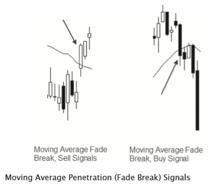
There are many ways to structure tests of moving averages. I did quite a few, but the one I want to share with you today I called the “Moving average penetration (Fade Break)” test. For a buy, the criteria are:

• Yesterday’s low was above the moving average
• Today’s close is below the moving average
• Buy on today’s close

You can see, the concept is that we are fading a close through the moving average. A visual may be helpful:

[Let me continue with some text from the unpublished portion of my book. (I already did the work once, so it makes sense to share it in its original form.) I’ll summarize at the end of this post.]

What happens after price breaks through a moving average? If moving averages are, in fact, important support or resistance levels, if large traders are making trading decisions based on the relationship of price to the average, we should see some reaction after the moving average fails to contain prices. It would be reasonable to assume that traders will exit or adjust positions on the break of the average, and this buying or selling pressure should cause distortions in the returns. We call this test the Moving Average Penetration test.

This set of conditions would have the trader always fading, or going against, price movements through a moving average: if price breaks below a moving average after being above it, this rule set will generate a buy signal. It is entirely possible that this is backwards, and perhaps these should be traded as breakouts by going with the direction of the price movement. Again, it does not matter; if the criteria are flipped for buy and sell signals, we will simply see negative excess returns for buys and positive for sells.

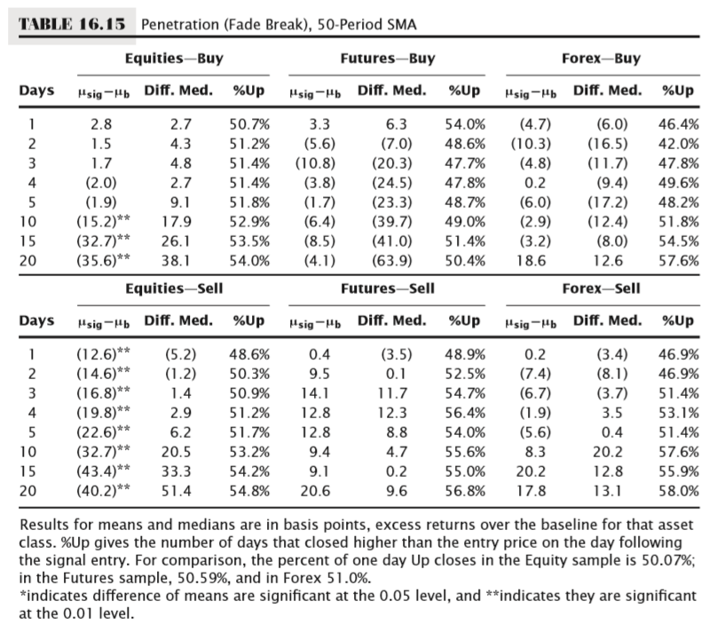
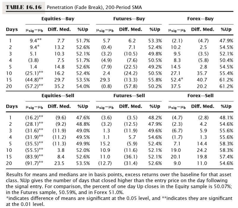
Fade test results

These results appear to be interesting, at least for the equities sample. The sell signals (which, remember, are based on shorting the first bar that closes above a moving average) show a consistent negative edge, and this edge is statistically significant. The buy signals also show an interesting pattern, but it is not as clear or as strong. The buys (again, this is buying the first bar that closes below a moving average) show an initial small positive edge that appears to decay into a negative edge between 5 to 10 days from the signal. This decay of a positive signal into a statistically significant sell signal may be a bit surprising; to better understand the dynamics involved we should ask if it could be due to the effect of a large outlier. Though the data is not reproduced in these tables, this effect does not seem to be attributable to a single outlier; when the equities universe is split into large-cap, mid-cap, and small-cap samples, the same signal decay is apparent in all market capitalization slices. If this were due to an aberration in a single stock, the decay would most likely be limited to a single market cap. It is also interesting to note that, while we have interesting patterns in equities, the futures and forex groups do not show any predictable pattern. This is the strongest clue we have had so far in these tests that perhaps not all assets trade the same from a quantitative perspective. If we continue to see evidence that assets behave differently, this would seem to present a significant challenge to the claims that all technical tools can be applied to any market or time frame with no adaptation.

The 200, 100, and 50 day averages are not special

Results from other tests, though not reproduced here, look very similar regardless of period (from 10 to 200) or type (exponential or simple) of moving average used in the test—the curious distortion in equity returns persists. Also, running the test on the random walk period moving average, not surprisingly, generates similar results. This might be a good place to pause and to think about what is going here. Based on these tests, we see absolutely no evidence validating moving averages as important levels. In the data and the results, we cannot distinguish between the different periods of moving averages: 20, 45, 50, 65, 150, 185, 200, 233, and any others basically all look the same. However, there is an unusual pattern in the Moving Average Penetration tests that warrants deeper investigation. Regardless of what moving average is used, there appears to be a statistically significant edge, at least in equities, for buying closes below and shorting closes above the moving average. Here is a radical thought: what happens if we repeat this test without the moving average?

No, it’s not the averages. It’s mean reversion.

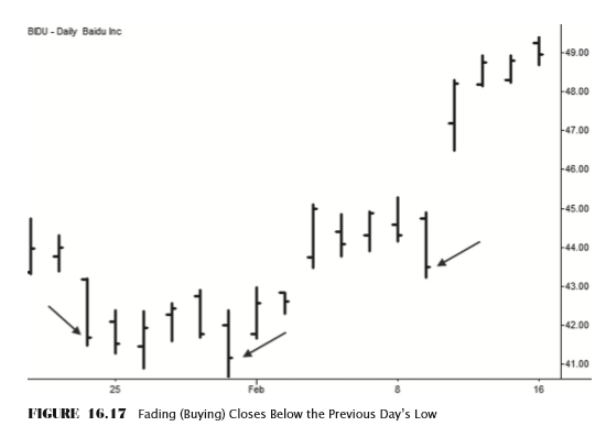
Yes, a test of moving averages without the average. Before you decide I have gone completely insane, consider the criteria for this Moving Average Penetration test. For a buy, price has to close below the average, and the previous bar’s low had to be above the average. In almost all cases, this means that the entry bar’s close is below yesterday’s low. Sure, it is possible that, in a few rare cases, the moving average could actually have risen enough that it is above yesterday’s low, but this is unlikely. It is far more likely that a close below the moving average is also a close below yesterday’s low. Figure 16.17 shows a graphical examples of fading a close outside the previous day’s range, and Table 16.17 presents summary statistics for this test.

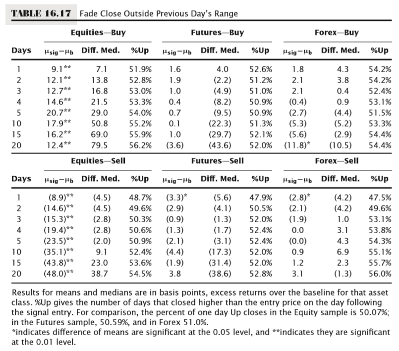
Now we are getting somewhere, and this is important, so make sure you understand this next point: First of all, these results look remarkably similar to the moving average breaks, at least for the first five days: Equities show a fairly large and statistically significant negative return after the sell condition. Equities also show a much smaller, but still significant, positive return following the buy condition. Though this is not conclusive evidence, it strongly suggests that the observed statistical edge around the moving average is simply a function of stocks’ tendency to reverse after a close outside of the previous day’s range. This is an expression of mean reversion, which is one of the verifiable, fundamental aspects of price movement.

It is also worth considering that what you see in Table 16.17 is significant on another level as well—these results strongly suggest that equities do not follow a random walk. Random walk markets would not show this anomaly. (Though the results are not presented here, in general, deviations of less than 2 basis points were seen from the baseline when this test was reproduced on random walk markets.) This is an extremely simple test with one criterion that produces a result that raises a serious challenge to one of the accepted academic hypotheses. We can say, based on this sample of 600 stocks over the past 10 years, that we find sufficient evidence to reject the random walk hypothesis for equities.

We’re not done yet, however. The situation for futures and forex is a bit more complicated. On one hand, there is a measurable difference in the proportion of positive closes on the first day after the signal. The Futures baseline closes up 50.6 percent of the time, compared to 52.6 percent and 47.9 percent for the buy and sell signals, respectively, and the forex baseline closes up 51.0 percent, compared to 54.2 percent and 47.5 percent for buy and sell signals. These differences are statistically significant, and could potentially give an edge in some situations. However, we have to note that the magnitude of the signal, in terms of deviation from the baseline, is very, very small. This is certainly too small to be economically significant on its own, but perhaps could be a head start when combined with some other factors. This is something we are going to see again and again in quantitative tests: futures and forex consistently tend to more closely approximate random walks than equities.

Conclusions and further lessons

This is just one test of many that I ran when I was looking at moving averages. You can play with this many different ways: what happens when the average breaks (as it has here), or holds? Does it matter if price moved a certain distance from the average? (Yes.) Do different periods or types of moving averages make a difference? (No.) And the questions go on.

As an interesting aside, I think I learned something new since doing this work a few years ago. I couldn’t quite understand the decay of the buy signal into a sell, or the strength of the overall effect of the sell. I think the reason is this: stocks tend to have stronger returns following closes in the top and bottom deciles of their range–that’s where a lot of the “juice” is. In addition, this sample is biased in that it did not have any companies that delisted or went bankrupt; the baseline adjustment methodology is one way to compensate for that bias, but we still may be picking up some asymmetry that biases the baseline too strongly positive. (This is speculation, but I spend a lot of time trying to shoot holes in my own tests!) At any rate, moving average events typically cluster somewhere closer to the median, so we are naturally picking up a lower set of returns in these events. More testing is necessary, but I think that’s a promising direction.

At any rate, there are a few important lessons here:

• There appear to be no special moving averages (100, 200, etc.) in stocks, futures, or currencies.
• Price touching or crossing a moving average does not appear to be a tradable event.
• We observe a small effect in stocks when a moving average breaks, but this effect is explainable through mean reversion.
• We have also seen evidence that not all asset classes trade the same. Again, this calls into question claims that any technical tool can be used on any asset or timeframe.

I apologize for the length of this post, but I received numerous requests for this information. If the information here is overwhelming, at least read the bullet point conclusions above a few times–those are critical, objective lessons that all technical traders should consider.