Blog

There is a lot of talk about the “historic bull market” we are in. Fundamental analysts raise valuation concerns, while technicians point to a myriad of factors, usually making the claim that we are in an unprecedented bull market and due for a reversal. This is simply not true.

Part of the problem comes from the common reliance on moving averages in this type of analysis, for example, pointing out that a stock index has been so many days above a moving average. While these statistics are easy to calculate and are objective true, the implications are never clearly examined. We are supposed to think, for instance, that a market that has been above a moving average for a long time is long overdue for correction. There is no evidence that shows that is true. ((E.g.,  try segregating market selloffs by the amount of time the market was above a moving average, or some other measure of “overboughtness”. Such tests fail to show an influence.)) It is easy to forget that price can come back to a moving average in one of two ways: either the price can decline to the average, or price can hold steady and the average will pull into price. Even if price does eventually come back to the moving average, there is no reason to assume the market will have gone down, and it is folly to think that the probabilities favor a selloff the longer a market is above an average.

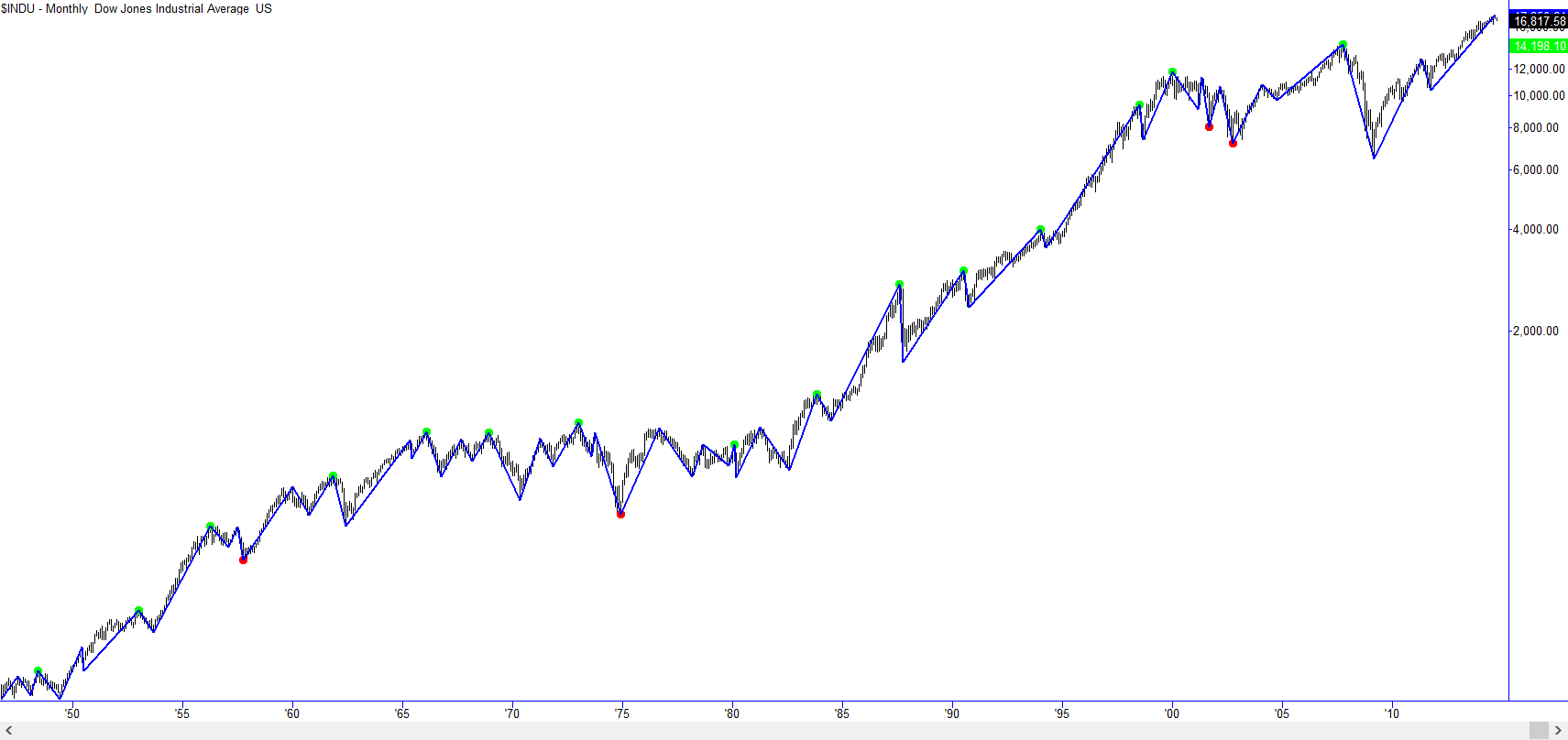
When we do any analysis, we must impose some structure on the market, but swing structure is clearly drawn from price without the addition of other calculations and tools–it is a very “pure” perspective on market structure. Take a look at the chart below, in which I’ve superimposed AlgoSwings on the monthly chart of the DJIA. AlgoSwings are calculated by a simple procedure:

• Find swing highs as an “isolated high”: the highest high of the preceding and following two bars. Do the same for swing lows. (We can use numbers other than two here.)
• Connect these highs and lows to give swings.
• Optional: filter out the very small swings by requiring a move of a certain number of ATRs from the previous swing. (This number can also be adjusted, or set to zero if you’d prefer no filter.)

You end up with a simple and robust measure of market swings:

Now, reconsider all the hype. When people talk about market history, sometimes they go back 20 years, but often less than 10. Simply by looking at markets back to the second World War, you now you have a bigger perspective than most journalists, commentators, and analysts. From a purely visual perspective ((remember, looking at a chart is not actual analysis!)) what does this chart look like? That’s right–business as usual, and certainly no sign of crazy, unsustainable overextension.

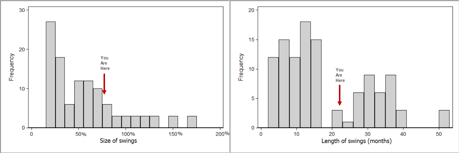
We can also consider the stats associated with these swings. In this case, this particular swing specification counts 230 swings, back to 1932. The average length of upswings was 17.3 months (standard deviation 12.7 months), and the average size of upswings was 54.8% (standard deviation 43.7%). ((The data is deliciously asymmetrical; downswings last an average of 7.9 months and only extend an average of -24.1%.)) The current upswing has gone on 24 months, for a gain of 66.8% from the previous swing low. This puts the current bull market in the 68th percentile for time and 70th for price–certainly not at all extreme.

It also can be instructive to look at the distributions of these measures.

Bottom line: we are in a bull market, but there is no technical (price-based or quantitative) reason to think that the market is overdue for a reversal. The current market is well within historical norms, and is not at all extreme. Ignore the noise and the hype, and focus on the message of the market.