Blog

Continuing on with the short series on backtesting in Excel, let’s look at some tools to visualize data and make some simple calculations. Excel is a good tool for quick and dirty data visualization in some cases–basic Excel graphs can be made quickly and show the relationships between simple series. I’ll end this post with a small challenge and encourage you to take the concepts presented to figure out how to create a moving average.

To get started, take the Excel sheet you have built from previous posts in the series, and delete rows so you have SPY and TLT close data for the dates 8/1/05 – 10/19/15. While it is not strictly necessary to do that, it will let you follow along more closely with what I am showing you here.

Simple graphs

Graphing data in Excel is simple:

1. Select the data you want to display in the graph. (Combination of shift/control/and arrow keys, but I’m trusting you have command of the tips and tools from previous posts.)
2. Go to the >Insert tab at the top of your version of Excel and select the chart type you want to insert. There are enough options for charts that I think it usually makes sense to do this from the menu bar rather than try to do it with keyboard shortcuts.
3. Theoretically, you should be able to select both the axis label and the data you want to display, but Excel may not guess what you are trying to do correctly. Most initial problems with Excel graphs can be fixed by right clicking on a blank space within the chart (i.e., not on the data lines, axis, etc.) and selecting the option >Select Data from the context menu that pops up. This menu allows you to not only select data but to edit those selections and tell Excel what, for instance, should be a label and what should be data. You’ll have to spend some time playing with this and perhaps doing a little research (use Google), but this will at least get you started in the right direction. The focus of this series is not on graphing, so I’m just going to leave you with the very first steps there.

First calculations

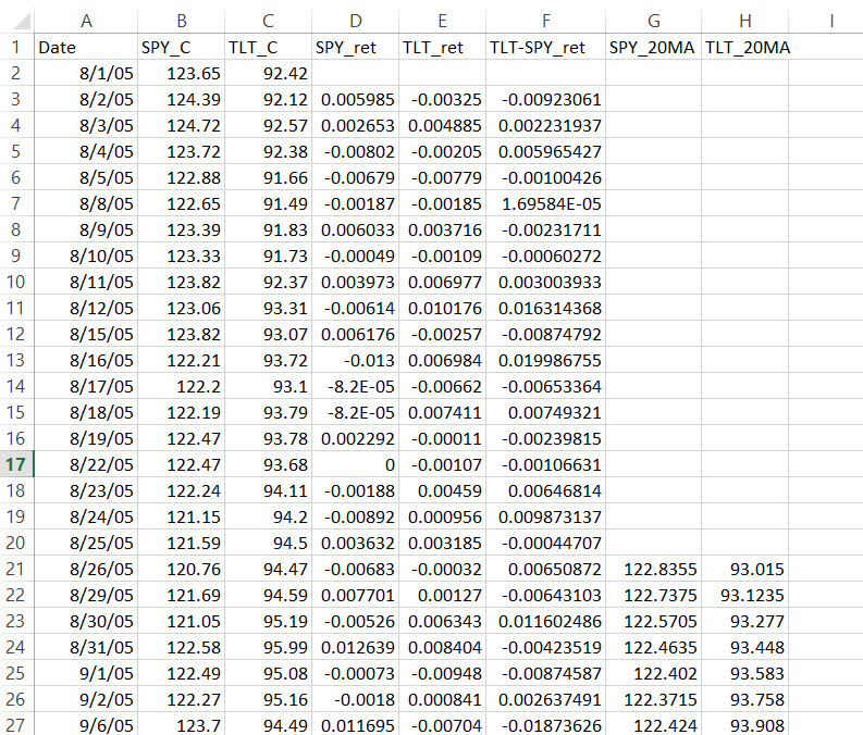
Remember, any calculation you want to make must begin with “=”. You can refer to other cells by their Letter/Number address most easily. So, if we go to cell D3 and type =B3/B2-1 we divide the SPY price on 8/2/05 by the price on 8/1/05 (previous day) and subtract one. (Normal order of operations applies, but for anything much more complicated than this, don’t hesitate to use parentheses.) This calculation gives us the percent change or return for SPY for 8/2/05. So far, not so interesting, but here is where the power of a spreadsheet starts to come through.

Now, select cell D3, tap Ctrl-C, and you should see “marching ants” confirming that this cell will be copied. Use down arrow to select cell E4, and tap Ctrl-V to paste the formula into the next cell. Now, you’ve just calculated the return for the SPY for the next day. Look at the formula you pasted which no longer refers to B3 and B2–as we copy down, the references move, so the it refers to B4 and B3. How would you calculate a return for TLT?

That’s right, you simply copy the cell over to the right, and the references will move a column over, now targeting TLT data for the same day instead of SPY. Now, copy both of those columns down to the bottom of the sheet, and, in a few keystrokes, you’ve calculated percentage returns for SPY and TLT for each day for many years. Maybe you are not ooh-ing and ah-ing over this exciting analysis so far, but this is the key to doing much more in-depth calculations in Excel–the fact that any calculation can be easily replicated.

One last thing, but it’s important: please label your columns. If you don’t do this it can make it very hard for you to understand what you’ve done and why you’ve done it. I’ve even come back to something I’ve done a few days later and had to spend a lot of time retracing my steps. Weeks later? Forget it; you’re basically starting over. Labels can help, and don’t be afraid to even write yourself notes in the sheet somehow. You’ll break this rule and you’ll be sorry you did. 🙂 For now, label column D SPY_ret, and column E TLT_ret.

Calculations on calculations

Another one of the strengths of using a spreadsheet is that you can easily break complex calculations down into component parts. Let’s say I want to put the excess return for TLT over SPY (defined as the return of TLT minus the return of SPY) for each day in column F. The correct formula is =(C3/C2-1)-(B3/B2-1), and spend a few moments making sure you understand that.

Now, this is a simple example, but we have basically two choices. You can create a formula like the one in the previous paragraph that does the calculations inside the cell, but this can be very hard to understand or troubleshoot. A better way is to do the component calculations in columns, and then simply refer to those partial answers. In this case, F3 can simply say =E3-D3 if you have been following along.

There are some stylistic issues here, and reasons you might prefer one solution over another. I’ve had cells that basically have so many steps in them they would be a full paragraph if printed, and that’s really bad practice. Try to get into the habit of breaking things up, as I’ve shown here, and use columns to do partial and preliminary calculations.

Homework

Some Excel formulas refer to a range, usually using this format (starting cell:ending cell). If we wanted to add cells A1 and A2 (we don’t, but just for sake of argument), the formula would be =SUM(A1:A2). Here’s a little homework question: the formula for average is… predictably… =AVERAGE(start:end). So, how would you create the 20 day moving averages of SPY and TLT price (not returns) in the picture below? We will pick up there tomorrow.